5.1 Basics of Linear Regression

Linear Regression really boils down to this simple equation.

\[ Y = b_0 + b_1 X \]

We want to predict \(Y\), our outcome variable or dependent variable (DV), using \(X\), which can have several names, like independent variable (IV), predictor or regressor.

\(b_0\) and \(b_1\) are parameters that we have to estimate in the model: \(b_0\) is the Constant or Intercept term, and \(b_1\) is generally called a regression coefficient, or the slope.

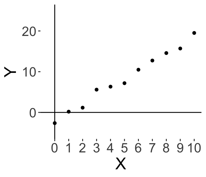
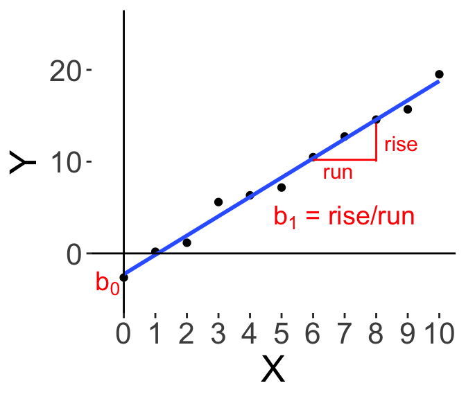
Below, we have a simple graphical illustration. Let’s say I have a dataset of \(X\) and \(Y\) values, and I plot a scatterplot of \(Y\) on the vertical axis and \(X\) on the horizontal. It’s convention that the dependent variable is always on the vertical axis.

On the right I’ve also drawn the “best-fit” line to the data. Graphically, \(b_0\) is where the line crosses the vertical axis (i.e., when \(X\) is 0), and \(b_1\) is the slope of the line. Some readers may have learnt this in high school, where the slope of the line is the “rise” over the “run”, so how many units of “Y” do we increase (‘rise’) as we increase “X”.

And that’s the basic idea. Our linear model is one way of trying to explain \(Y\) using \(X\), which is by multiplying \(X\) by the regression coefficient \(b_1\) and adding a constant \(b_0\). It’s so simple, yet, it is a very powerful and widely used tool, and we shall see more over the rest of this chapter and the next few chapters.

Our dependent variable \(Y\) is always the quantity that we are interested in and that we are trying to predict. Our independent variables \(X\) are variables that we use to predict \(Y\).

Here are some examples:

Dependent Variable Y	Independent Variable X
Income	Years of Education
Quartly Revenue	Expenditure on Marketing
Quantity of Products Sold	Month of Year
Click-through rate	Colour of advertisement (Note that this is an experiment!)

Perhaps we are interested in predicting an individual’s income based on their years of education. Or for a company, we might want to predict Quarterly Revenue using the amount we spent on Marketing, or predict sales at in different months of the year.

We can also use regression to model the results of experiments. For example, we might be interested in whether changing the colour of an advertisement will affect how effective it is, measured by how many people click on the advertisement (called the click-through rate, measuring how many people click on our ad). So we may show some of our participants the ad in blue, some in green, etc, and then see how that affects our click-through rate. So linear modelling can and is frequently used to model experiments as well.

Independent Variables can be continuous (e.g., Years; Expenditure), or they can also be discrete/categorical (e.g., Month, Colour, Ethnicity). And we shall see examples of both in this chapter

Similarly, Dependent Variables can either be continuous or categorical. In this Chapter we shall only cover continuous DVs, and we shall learn about categorical DVs in the next Chapter on Logistic Regression.