14.6 Sensitivity Analysis
When we get an optimal solution to a linear optimisation problem, oftentimes we may want to ask: what if we change the objective by a little, or what if we change the constraints by a little, what would happen? i.e., how sensitive is the solution to changes in the problem?
Sensitivity analysis allows us to ask this question systematically. Here we shall cover two types of sensitivity analyses – varying objective function coefficients, and varying constraint values.
Varying objective function coefficients
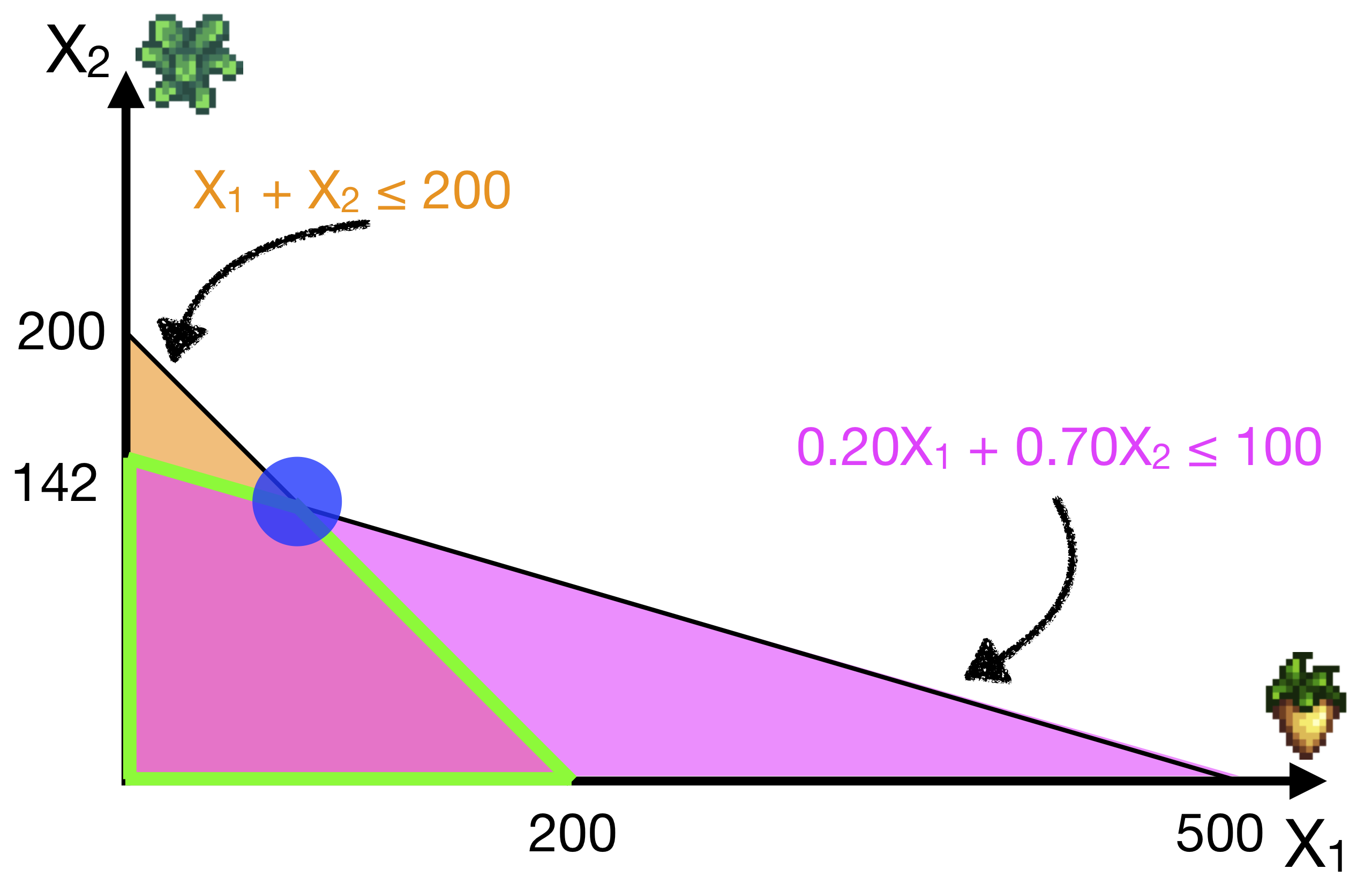
Recall our farming example: our optimal solution is \(X_1\) = 80, \(X_2\) = 120, and our objective function is: \[ \text{Profit} = 0.15 X_1 + 0.40 X_2 \]
What if Farmer Jean’s customer decides to reduce the amount they are willing to pay for Kale (\(X_2\)) to $1.00 (reducing Jean’s profits from 0.40 to 0.30 per unit of \(X_2\)). \[ \text{Profit} = 0.15 X_1 + \color{red}{0.30} X_2 \]
Will that change our optimal solution?
Turns out, no, it doesn’t. (Try running the code again to verify that the optimal solution is still (80,120)!)
But now if the price that Farmer Jean can sell Parsnips (\(X_1\)) drops from 0.35 to 0.30, i.e., reducing her profits per unit-parsnips from 0.15 to 0.10,
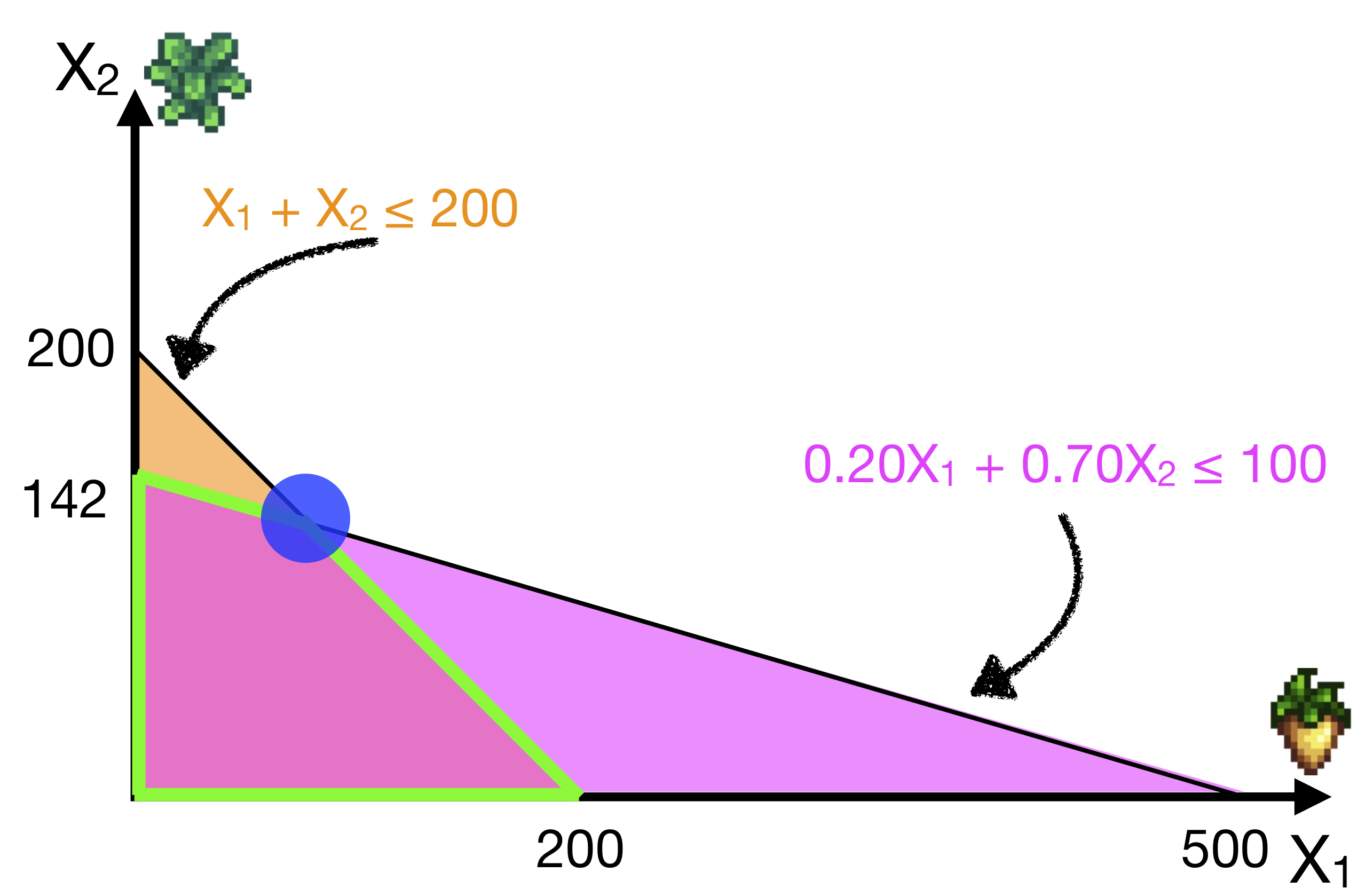
\[ \text{Profit} = \color{red}{0.10} X_1 + 0.40 X_2 \] Then the optimal solution actually changes (to \(X_1\) = 0, \(X_2\) = 142)! Basically, Parsnips are now not profitable, and Jean should plant plant all Kale.
Graphically the optimal solution now moves from the blue vertex to the green vertex. The optimal solution is to produce as much Kale as she can afford.
Indeed in the first case, reducing the price of \(X_2\) by 10 cents did not change the solution, but in the second case, reducing the price of \(X_1\) by 5 cents did! So this solution is sensitive to some changes but not others.
Varying objective function coefficients in R
R’s lpSolve::lp() function helps you to calculate the range of coefficient values for which the given solution is still optimal. So again, recall that the original objective function is:
\[ \text{Profit} = 0.15 X_1 + 0.40 X_2 \]
We use lp.solution$sens.coef.from and lp.solution$sens.coef.to to get the range of coefficients.
## [1] 0.1142857 0.1500000## [1] 0.400 0.525The way you read this is that “from” is the lower bound of the coefficients (\(X_1\) and \(X_2\) respectively), while “to” gives the upper bound of the coefficients.
- This means that as long as the coefficient on \(X_1\) lies between [0.1143, 0.400], this solution is still optimal.
- Or if the coefficient on \(X_2\) lies between [0.150, 0.525], this solution is still optimal.
If the coefficients shift outside these ranges, then the solution will move to a different vertex. (How will they move?)
Note that all of these sensitivity calculations assume you only adjust one coefficient at a time. This means that if you decide to reduce \(X_1\) to 0.12 and increase \(X_2\) to 0.50, the optimal solution might change. These ranges assume that you only change that one coefficient while holding the rest constant. If you want to change two or more coefficients, you should re-run the model.
Now let’s think through and try to predict what happens when these coefficients go out of these bounds. We just saw that if the coefficient on \(X_1\) goes to 0.10, which is less than 0.1143, then the solution moves to: produce no \(X_1\) and produce maximum \(X_2\).
What if the coefficient on \(X_1\) goes above 0.400? What do you think will happen? Increasing the profit of \(X_1\) beyond this range should mean that it has become more profitable to produce \(X_1\), and we know that the solution must lie on a vertex, so we move down the edge of the feasible region to the solution on the horizontal axis, \(X_1 = 200, X_2 = 0\).
Similarly, we can think about what will happen when the coefficient on \(X_2\) drops below 0.15: it becomes not profitable to produce Kale, so we’ll also get the point \(X_1 = 200, X_2 = 0\). But when the coefficient on \(X_2\) rises above 0.525, then it becomes much more profitable to produce Kale, so we’ll come to the solution \(X_1 = 0, X_2 = 142\).
Varying Constraint Values (Shadow Prices)
The next type of sensitivity analysis we shall look at is what happens when we vary the constraint values.
We’ll introduce a new term called shadow prices. The Shadow Price of a constraint is the change in the objective function value per unit-increase in the right-hand-side value of that constraint (holding all else equal). Let’s break this down.
In the Farming example, we have two constraints.
Let’s consider the first constraint. What if we increased the RHS of the first constraint from 100 to 101?
\[0.20X_1 + 0.70X_2 \leq 100 \quad \rightarrow \quad 0.20X_1 + 0.70X_2 \leq \color{green}{101}\]
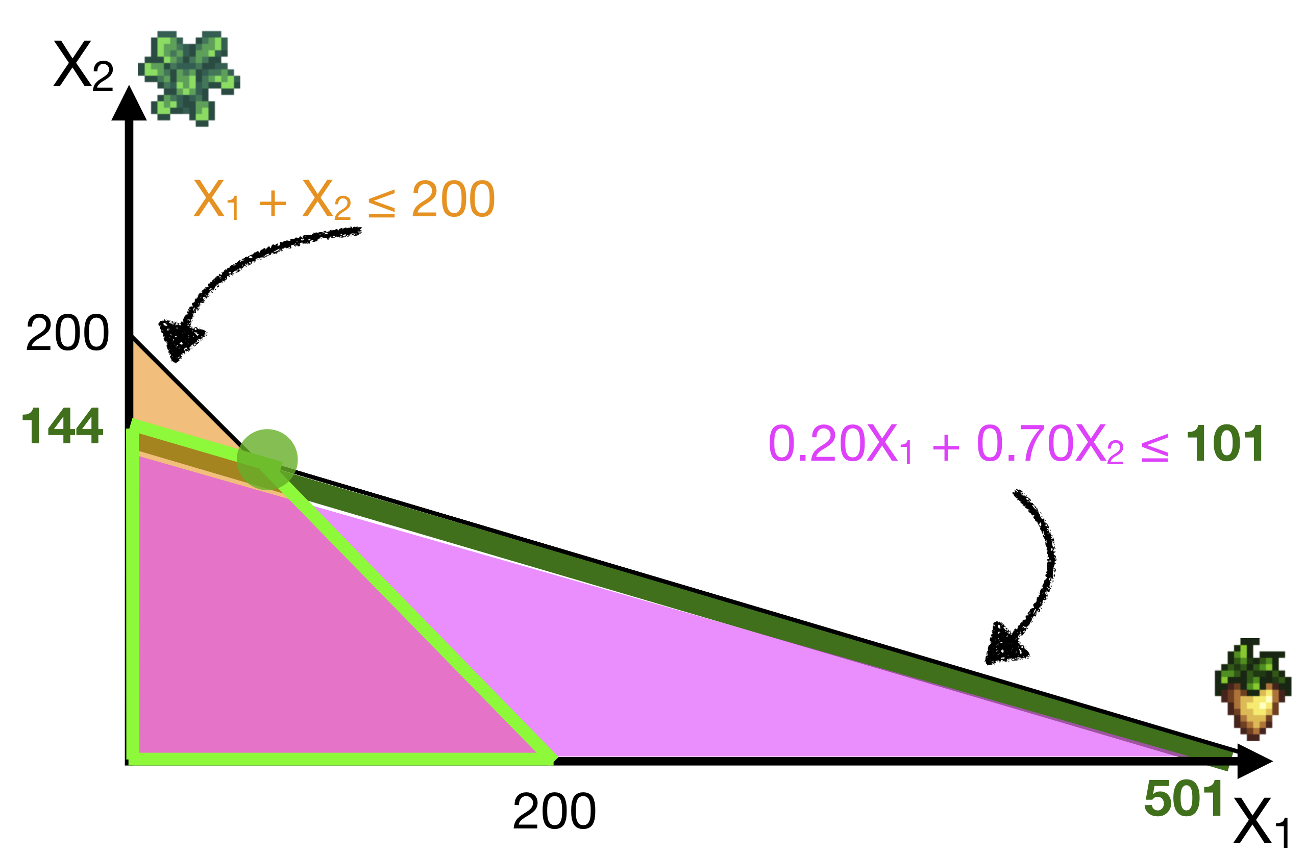
The feasible region was pushed outwards a little, by adding this green segment. Doing this will move the optimal vertex up and to the left.
The new solution is (\(X_1\) = 78, \(X_2\) = 122), which gives a profit of $60.50 – an increase of $0.50
Thus, increasing the budgetary constraint by 1 unit (100 to 101) increases the profit by $0.50 (from $60 to $60.50). Hence, (by definition), the Shadow Price of the first constraint is $0.50.
What this means is that if Farmer Jean increased her operating budget from $100 to $101, then she can increase her profits by $0.50. That’s a pretty good return-on-investment! (Note that the optimal solution also changes, but here the shadow price indicates the effect of changing the constraint value on the PROFIT).
Next, let’s consider the second constraint. What if we increased the RHS of the second constraint from 200 to 201?
\[X_1 + X_2 \leq 200 \quad \rightarrow \quad X_1 + X_2 \leq \color{cyan}{201}\]
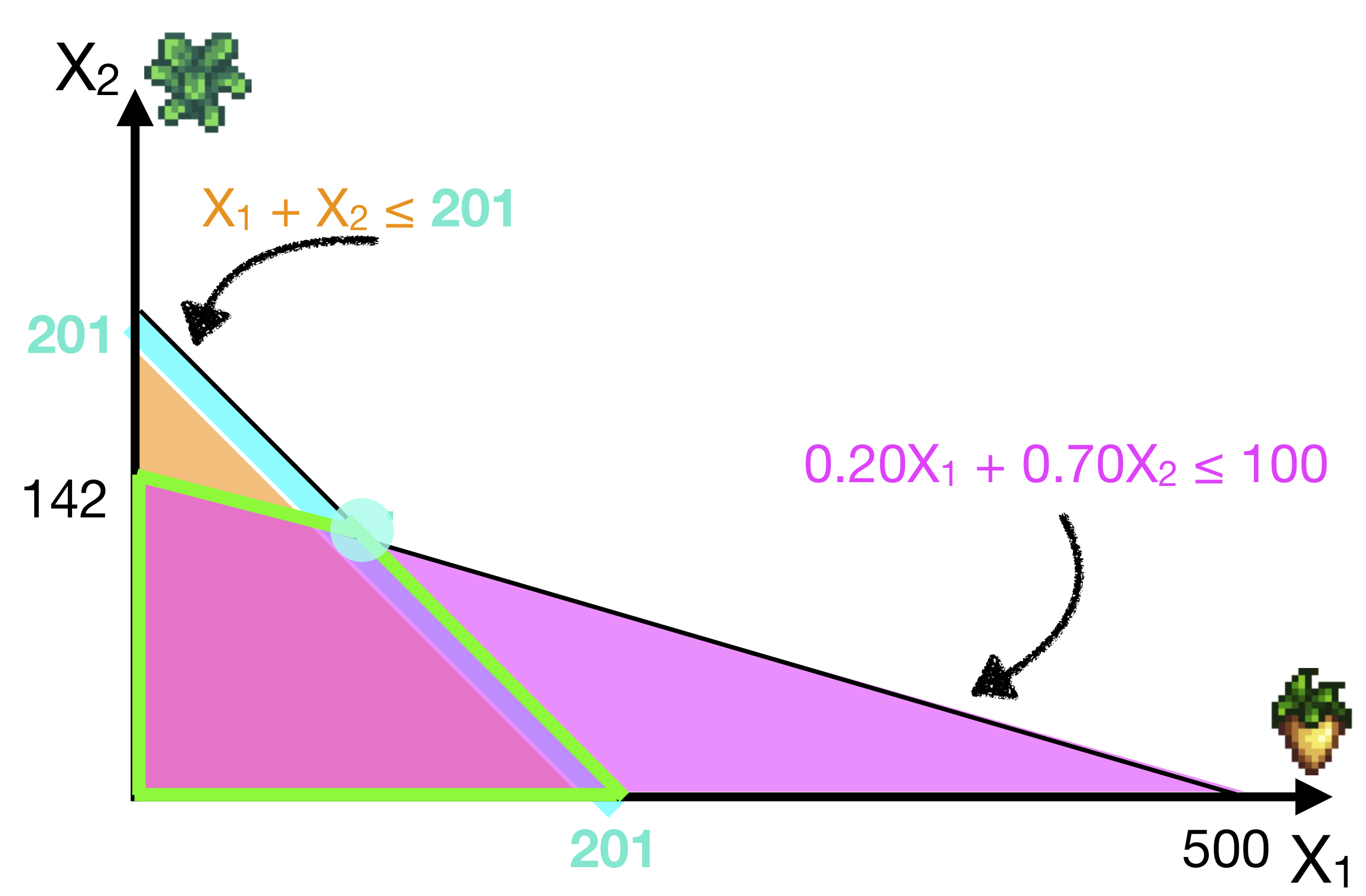
The feasible region was pushed out a little, by adding this cyan segment, which moved the optimal vertex down and to the right.
The new solution is (\(X_1\) = 81.4, \(X_2\) = 119.6), which gives a profit of $60.05 – an increase by $0.05
Thus, increasing the space constraint by 1 unit (200 to 201) increases the profit by $0.05 (from $60 to $60.05). The Shadow Price of the space constraint is $0.05.
What this means is that if Farmer Jean increased her land plot size from 200 to 201, then she can increase her profits by $0.05. That’s not as high as the budgetary constraints, so this translates to a good recommendation: if Jean wants to increase her profit, she gets more bang of the buck if she gets more operating budget than land space.
Varying Constraint Values in R
Shadow prices are also known as duals in other fields (e.g. computer science), so we use lp.solution$duals to get them.
## [1] 0.50 0.05 0.00 0.00Notice that there are four values here. The first two are the two constraints we put in, in the order they were specified in the constraints matrix (so \(0.20X_1 + 0.70X_2 \leq 100\) then \(X_1 + X_2 \leq 200\)). So we can see, as per our calculations above, that the shadow price of the first constraint is $0.50, and that of the second constraint is $0.05.
The last two are the shadow prices of the non-negativity constraints \(X_1 \geq 0\), and \(X_2 \geq 0\). This means that the change in the optimal profit, if we were to increase the right hand side values from 0 to 1, are both 0. Note that in some fields, the shadow prices of the non-negativity constraints have a special name, reduced costs. But the interpretation is the same.
Why would we have a shadow price of zero for these non-negativity constraints? In this particular case, in the optimal solution we are already producing non-zero quantities of \(X_1\) and \(X_2\). Thus, increasing the right-hand-side value (i.e., forcing us to produce at least 1 \(X_1\) or at least 1 \(X_2\)) will not change our optimal solution. The shadow prices are zero.
Binding vs non-binding constraints
In general, constraints can either be binding or non-binding for the optimal solution. Constraints that are binding ‘restrict’ the optimal solution; so in the Parsnips/Kale example, both the Budget and Space constraints are binding; if we increase the right-hand-side of the constraints, we can do better and increase our profit. Hence, they have non-zero shadow prices.
Conversely, non-binding constraints do not restrict or bind the optimal solution. Thus, even if we change the right-hand-side value of the constraint by 1, we will not affect the optimal solution. Thus, shadow prices are zero for non-binding constraints.
In certain cases, we might even have negative shadow prices. Let’s consider a modified objective function in the same Parsnip-Kale example, where the profit of Kale is increased to 0.53.
\[ \text{Profit} = 0.15 X_1 + \color{red}{0.53} X_2 \]
We saw from our earlier sensitivity analysis that this will change the optimal solution to: \(X_1 = 0, X_2 = 142\). Let’s check this by re-running this modified linear optimization problem, saving it as lp.solution2:
# defining parameters
objective.fn2 <- c(0.15, 0.53)
const.mat <- matrix(c(0.20, 0.70, 1, 1) , ncol=2 , byrow=TRUE)
const.dir <- c("<=", "<=")
const.rhs <- c(100, 200)
# solving model
lp.solution2 <- lp("max", objective.fn2, const.mat,
                   const.dir, const.rhs, compute.sens=TRUE)


# check if it was successful; it also prints out the objective fn value
lp.solution2
## Success: the objective function is 75.71429# Printing it out:
cat("The optimal solution is:", lp.solution2$solution, "\nThe optimal objective function value is:", lp.solution2$objval, "\nwith the following Shadow Prices", lp.solution2$duals)## The optimal solution is: 0 142.8571
## The optimal objective function value is: 75.71429
## with the following Shadow Prices 0.7571429 0 -0.001428571 0As we expected, the solution is \(X_1 = 0, X_2 = 142\) (rounded down). Now, if we look at the shadow prices, we notice that the shadow price of the first constraint: \(0.20X_1 + 0.70X_2 \leq 100\), is +0.75, so increasing the budget by $1 will increase profits by $0.75. The shadow price of the second constraint, \(X_1 + X_2 \leq 200\), in this case, is 0. We can also see that because the total amount of land used \(X_1 + X_2 = 0 + 142 = 142\) is much less than the available budget, this constraint now becomes non-binding at this solution, and hence the shadow price of this constraint is zero. Getting access to more land will not help improve profits.
But wait, the third shadow price returned by lp.solution2$duals is negative! What does that mean? This shadow price corresponds to the non-negativity constraint \(X_1 \geq 0\). Going by the definition of the shadow price, this means that increasing the value of the right hand side of this constraint, to \(X_1 \geq \color{red}{1}\) will reduce the optimum profit by -$0.0014. This is because if this constraint were to be changed, then now we are forced to produce at least 1 unit of \(X_1\), which is now less profitable, and hence total profit should go down.
Finally, note that this also implies that \(X_1 \geq 0\) is a binding constraint, because changing the value of this constraint will affect the optimal solution. So binding constraints can have either positive, or negative, shadow prices.
Summarizing sensitivity analyses
Solving an optimization problem is straight-forward once you have the objective function and the constraints. Getting the optimal solution is not the end of it. As a top-notch business analyst, we can add more value to the business decision by doing and interpreting sensitivity analyses.
- We can examine the range of coefficients over which this solution is valid, and make recommendations. For example, we saw earlier than if the profit of Kale goes above 0.53 or profit per Parsnip goes below 0.11, then it makes more sense to switch to producing as much Kale as possible.
- For example, you could provide the following recommendation to Farmer Jean: “If the profit per unit-Kale goes above $0.53 or if the profit per unit-Parsnips goes below $0.11, then please switch your whole production to Kale.”
- Secondly, we can examine and interpret shadow prices:
- For example, to Farmer Jean: “If you get one additional plot of land, you can make $0.05 more profit. But if you get $1 more of budget to buy crops, you can increase your profit by $0.50 (by changing your planting allocation to …)”
More broadly, as analysts we could run “what-if” analyses to study the impact of getting more resources, of changing our prices, and of many other possible business decisions. These type of analyses require much more experience, but are potentially much more valuable to making better business decisions.