6.3 Examples: Logistic Regression
Let’s consider a classic dataset from the ill-fated maiden voyage of the RMS Titanic in 1912, which is available in R. First let’s load in the R package (library(titanic), installing it if it doesn’t already exist on your system), and use the data frame called titanic_train. We first inspect the data frame to get a sense of the variables.
## Warning: package 'titanic' was built under R version 4.0.2## let's use the dataset called titanic_train
# inspect the first two rows: we see the data frame has variables PassengerId, Survived, Pclass, Name, Sex, Age, SibSp, Parch, Ticket, Fare, Cabin, and Embarked
head(titanic_train, 2)## PassengerId Survived Pclass
## 1 1 0 3
## 2 2 1 1
## Name Sex Age SibSp Parch
## 1 Braund, Mr. Owen Harris male 22 1 0
## 2 Cumings, Mrs. John Bradley (Florence Briggs Thayer) female 38 1 0
## Ticket Fare Cabin Embarked
## 1 A/5 21171 7.2500 S
## 2 PC 17599 71.2833 C85 C## [1] 891##
## 0 1
## 549 342##
## female male
## 314 577So we can see that the dataset contains 891 observations (passengers) with 12 variables. We’ll just look at a few of these variables.
Of these 891 passengers, 342 passengers survived the sinking of the Titanic (Survived=1), while 549 did not (Survived=0). And of these 891 passengers, 314 were female (Sex="female"), while 577 were male (Sex="male").
Let’s estimate a model to predict Survived from Sex and Age. That is, can we predict a passenger’s chance of survival given their sex and age?
First, as usual let’s visualize our data
How do we visualize Survived, which is a binary variable that takes on values {0, 1}, as well as Sex, which is another binary variable that takes on values {male, female}? There are many different types of visualizations, but below we’ll use a stacked bar plot:
# munging, then plotting
titanic_table <- titanic_train %>%
                  group_by(Survived, Sex) %>%
                  summarize(number=n()) %>%
                  mutate(Survived = factor(Survived,
                                           levels=c(0,1), labels=c("No", "Yes")))
## `summarise()` regrouping output by 'Survived' (override with `.groups` argument)ggplot(titanic_table, aes(x=Sex, y=number, fill=Survived)) +
geom_bar(stat = "identity") + ylab("Number of passengers") + theme_bw()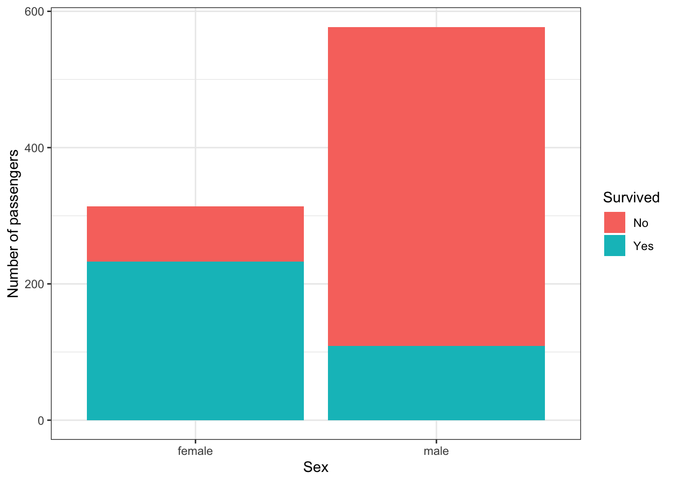
The blue bars show the number of passengers who survived, and red indicates the number of passengers who did not survive. On the left we plot female passengers, and on the right, male passengers.
So first, we notice (i) there were more male passengers than female passengers, (ii) that of the female passengers, there were more passengers that survived than passengers than did not survive (blue bar is larger than the red bar), and (iii) of the male passengers, there were more passengers that did not survive than those who did (red bar is larger than blue bar).
Ok on to the actual regression. Let’s estimate the model and inspect the summary of the model:
# running a logistic regression via a general linear model
fit_log1 <- glm(Survived ~ Sex + Age, family="binomial", titanic_train)

summary(fit_log1)
##
## Call:
## glm(formula = Survived ~ Sex + Age, family = "binomial", data = titanic_train)
##
## Deviance Residuals:
## Min 1Q Median 3Q Max
## -1.7405 -0.6885 -0.6558 0.7533 1.8989
##
## Coefficients:
## Estimate Std. Error z value Pr(>|z|)
## (Intercept) 1.277273 0.230169 5.549 2.87e-08 ***
## Sexmale -2.465920 0.185384 -13.302 < 2e-16 ***
## Age -0.005426 0.006310 -0.860 0.39
## ---
## Signif. codes: 0 '***' 0.001 '**' 0.01 '*' 0.05 '.' 0.1 ' ' 1
##
## (Dispersion parameter for binomial family taken to be 1)
##
## Null deviance: 964.52 on 713 degrees of freedom
## Residual deviance: 749.96 on 711 degrees of freedom
## (177 observations deleted due to missingness)
## AIC: 755.96
##
## Number of Fisher Scoring iterations: 4Let’s interpret the coefficients. Let’s write out the equation: \[\text{logit}( \text{Survived} ) = b_0 + b_\text{Sex} X_\text{Sex} + b_\text{Age} X_\text{Age}\]
- where \(X_\text{Sex}\) is a binary variable. Recall that
Ruses dummy coding, and from inspecting the summary we can also see thatfemaleis the reference group, soX_\text{Sex} = 1if male and0if female. - and \(X_\text{Age}\) is a real-valued number.
If we plug the numbers in, we get:
\[\text{logit}( \text{Survived} ) = 1.2773 - 2.4659 X_\text{Sex} - 0.0054 X_\text{Age}\]
So let’s interpret:
- (intercept, or \(b_0\)): Log-odds of
Survivedwhen \(X_\text{Sex}\) and \(X_\text{Age}\) are both zero.- In English: The predicted odds of survival of a female, 0-year old person = \(exp(1.2773) = 3.59\).
- (\(b_\text{Sex}\)): Expected increase in log-odds of
Survivedwhen \(X_\text{Sex}\) becomes 1, holding \(X_\text{Age}\) constant.- In English: A male passenger, compared to a female counterpart of the same age, has a decreased log-odds of survival of 2.466 (\(b_\text{Sex}\))
- Alternatively, being male would multiplies the odds of survival by \(exp(-2.466) = 0.085\). Thus the odds of survival for males decrease to 0.085x that of females.
- i.e., holding age constant, male passengers’ odds of survival are 0.085 times that of female passengers.
- Let’s plug some numbers in to check:
- When \(X_\text{Sex}\) and \(X_\text{Age}\) are 0, the odds are \(exp(1.277) = 3.59\)
- If we now increase \(X_\text{Sex}\) to 1, the odds are now \(exp(1.277 -2.466) = 0.305\)
- The odds have decreased by \((0.305)/3.59 \sim 0.085\) times
- Note that we can discuss the coefficient interpretations in terms of log-odds, or odds. But these numbers do not reflect probability!
- (\(b_\text{Age}\)): Expected increase in log-odds of event per unit-increase of \(X_\text{Age}\), holding \(X_\text{Sex}\) constant.
- Try writing this interpretation out in English!