5.5 Examples: Simple Regression

Here’s a simple example to illustrate what we’ve discussed so far, by using a dataset that comes bundled with R, the mtcars dataset. We can load the dataset using data(mtcars).

First, let’s see what the data looks like, using head(mtcars), which prints out the first 6 rows of mtcars.

data(mtcars)
head(mtcars)

##                    mpg cyl disp  hp drat    wt  qsec vs am gear carb
## Mazda RX4         21.0   6  160 110 3.90 2.620 16.46  0  1    4    4
## Mazda RX4 Wag     21.0   6  160 110 3.90 2.875 17.02  0  1    4    4
## Datsun 710        22.8   4  108  93 3.85 2.320 18.61  1  1    4    1
## Hornet 4 Drive    21.4   6  258 110 3.08 3.215 19.44  1  0    3    1
## Hornet Sportabout 18.7   8  360 175 3.15 3.440 17.02  0  0    3    2
## Valiant           18.1   6  225 105 2.76 3.460 20.22  1  0    3    1

We’re interested in particular in predicting the fuel economy (mtcars$mpg, measured in miles per gallon) of certain vehicles using its horsepower (mtcars$hp).

Let’s plot what they look like on a scatterplot.

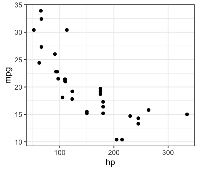
ggplot(mtcars, aes(x=hp, y=mpg)) + geom_point() + theme_bw()

It looks like there is a linear trend! We can see visually that as horsepower increases, fuel economy drops; large cars tend to guzzle more fuel than smaller ones. And finally, we can run the linear model using using lm(mpg ~ hp, mtcars):

summary(lm(mpg ~ hp, mtcars))

## 
## Call:
## lm(formula = mpg ~ hp, data = mtcars)
## 
## Residuals:
##     Min      1Q  Median      3Q     Max 
## -5.7121 -2.1122 -0.8854  1.5819  8.2360 
## 
## Coefficients:
##             Estimate Std. Error t value Pr(>|t|)    
## (Intercept) 30.09886    1.63392  18.421  < 2e-16 ***
## hp          -0.06823    0.01012  -6.742 1.79e-07 ***
## ---
## Signif. codes:  0 '***' 0.001 '**' 0.01 '*' 0.05 '.' 0.1 ' ' 1
## 
## Residual standard error: 3.863 on 30 degrees of freedom
## Multiple R-squared:  0.6024, Adjusted R-squared:  0.5892 
## F-statistic: 45.46 on 1 and 30 DF,  p-value: 1.788e-07

Looking at the coefficient table, we can see that $b_0$, the intercept term, suggests suggests that, according to our model, a car with zero horsepower (if such a vehicle exists) would have a mean fuel economy of 30 mpg.

We can look at the coefficient on $X$, which is $b_1 = -0.068$. Now this means that every unit-increase in horsepower would be associated with a decrease in fuel efficiency by -0.068 miles per gallon. Now, these are quite strange units to think about: for one, we do not think about horsepower in 1’s and 2’s; we think of horsepower in the tens or hundreds, and typical cars have horsepowers around 120 (the median in our dataset is 123). Secondly, -0.068 miles per gallon sounds pretty little, given that we see in the data that the mean fuel consumption is about 20 mpg.

What we can do to help our interpretation is to multiply our coefficient to get more human-understandable values. This means that, according to the model, an increase of horsepower by 100 units, will be associated with a decrease in fuel efficiency by 6.8 miles per gallon. Ahh these numbers make more sense now.

Finally, we note that the $R^2$ of this model is 0.6024. This means that the model explains about 60% of the variance in the data. Again, it’s hard to objectively say whether this is amazing or still needs more work, because this really depends on our desired context.

One takeaway from this example is that the linear model just calculates the coefficients based upon the numbers that we, as the analyst, provide it. It is up to us to then read the numbers that are output from the model, and make sense of those numbers, and interpret the meaning of those numbers. So this means being aware of units, and also not hesitating to wonder, “hmm this isn’t right, did I code everything correctly?”