13.1 Time Series Basics
First, let’s introduce some useful terminology that we can use to describe time-series data.
Trend: a gradual upward or downwards movement of a time series over time.
A Seasonal effect: an effect that occurs/repeats at a fixed interval
- Could be at any time-scales
- Examples: Diurnal temperature, temperature and length of day in temperate climates, “holiday season sales” that occur at specific times in the year
Cyclical effects: longer-term effects that do not have a fixed interval/length
- Example: stock market “boom/bust cycles”.
- The difference between cyclical and seasonal effects is that the latter are predictable, in that they repeat at regular intervals.
Stationarity: when statistical properties of the time-series (e.g., mean, variance) do not change over time.
- So by definition, a stationary time-series has no trend.
Autocorrelation: when a time-series is correlated with a past version of itself
- Auto here means “with itself”, and so autocorrelation means that the signal Y is correlated with previous versions of itself.
Here are some examples to motivate how time-series data is interesting:
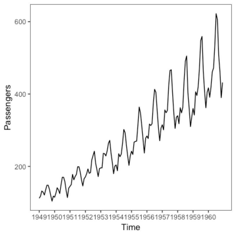
Here we have a dataset, which is in base R and which shows the monthly total of international airline passengers from 1949 to 1960. You can see that there is a gradual increase, but there is also this very stable pattern, going up and down over a year. Thus, this dataset shows a trend, and an obvious seasonal effect.
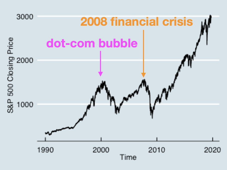
This is a graph showing the historical prices of the S&P500, a stock market index listed on the stock exchanges in the US, from 1990 until 2019. There are a lot of things going on, as is the case in real world data: There is a dramatic increase in price in the past 3 decades (trend), but also these large stock market fluctuations, or cycles.
The first of these cycles was the dot-com bubble in the 2000s, when tech companies were getting very hot, the internet was opening up, everyone was investing heavily in dot-com companies. The nature of these bubbles, however, is not that there is no value, but that the value is overestimated and actually doesn’t match the risks or the actual return-on-investment. So when investors started realising this and when companies actually couldn’t deliver as much as they promised, the bubble popped and the stock market crashed. This second cycle here precipitated what the 2008 financial crisis, and was actually due to overvalued mortgage loans in the US. Part of the American dream was to be able to own your own house in the suburbs; banks capitalized on this and started offering generous loans to people who couldn’t really afford them, and who were in turn more likely to default on paying their loans. This resulted in a “housing bubble”. When people actually started defaulting on their loans, the banks actually started losing money and some went bankrupt, and the whole worldwide economy was impacted.
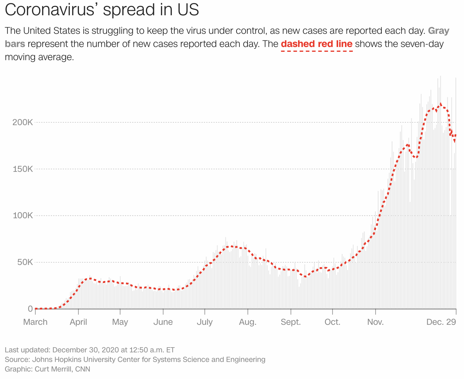
Finally, here’s another time-series graph that is relevant given the Covid-19 pandemic. This screenshot, taken from CNN on Dec 30, 2020, contains the number of cases in the US up through Dec 29 of 2020. (I note that the data is publically available, while credits for this particular visualization goes to CNN.) Similar to the stock market example, there is both an increasing trend, as well as several cycles.