13.2 Smoothing-based models
Time-series data is often quite noisy, and often we may want to “smooth” out individual variation in the data, in order to be able to see the bigger picture, like trends.
First we define a simple moving average window, sometimes called a sliding window: we define a \(k\)-period simple moving average window as just the average of the most recent \(k\) elements of the time-series:
\[\text{Window}_t = \frac{1}{k} \left( Y_t + Y_{t-1} + \ldots + Y_{t-(k-1)} \right)\]
Note that the default for early timepoints (when there’s not enough to fit in the window), is undefined, and in R is left as a missing, or NA value. There are several functions you can use to calculate these moving averages, here we use the SMA function from the TTR package:
# There are many different ways to calculate simple moving averages.
# Here's one from the TTR package
# install.packages('TTR')
library(TTR)
SMA(df$y, n=3) # taking window size of 3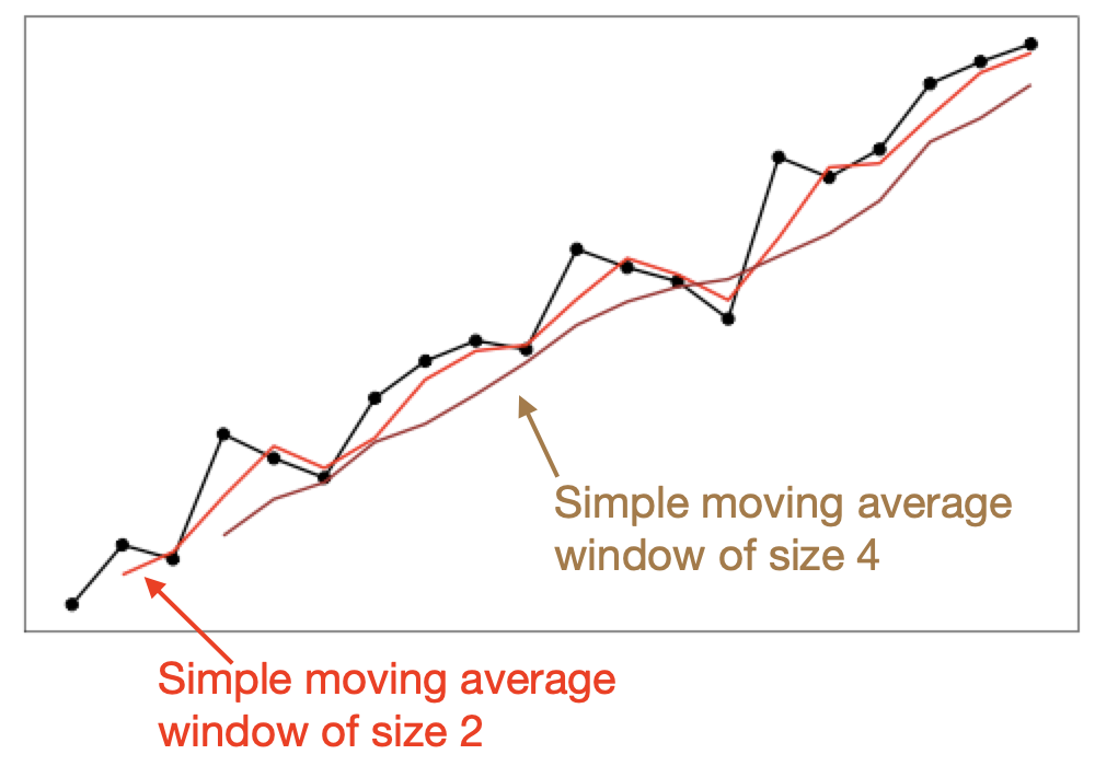 This graph shows a simple time-series (in black), as well as the corresponding simple moving average windows of size 2 (in red) and size 4 (in brown). Take a minute to look at how the windows “smooth” out the variation in the data.
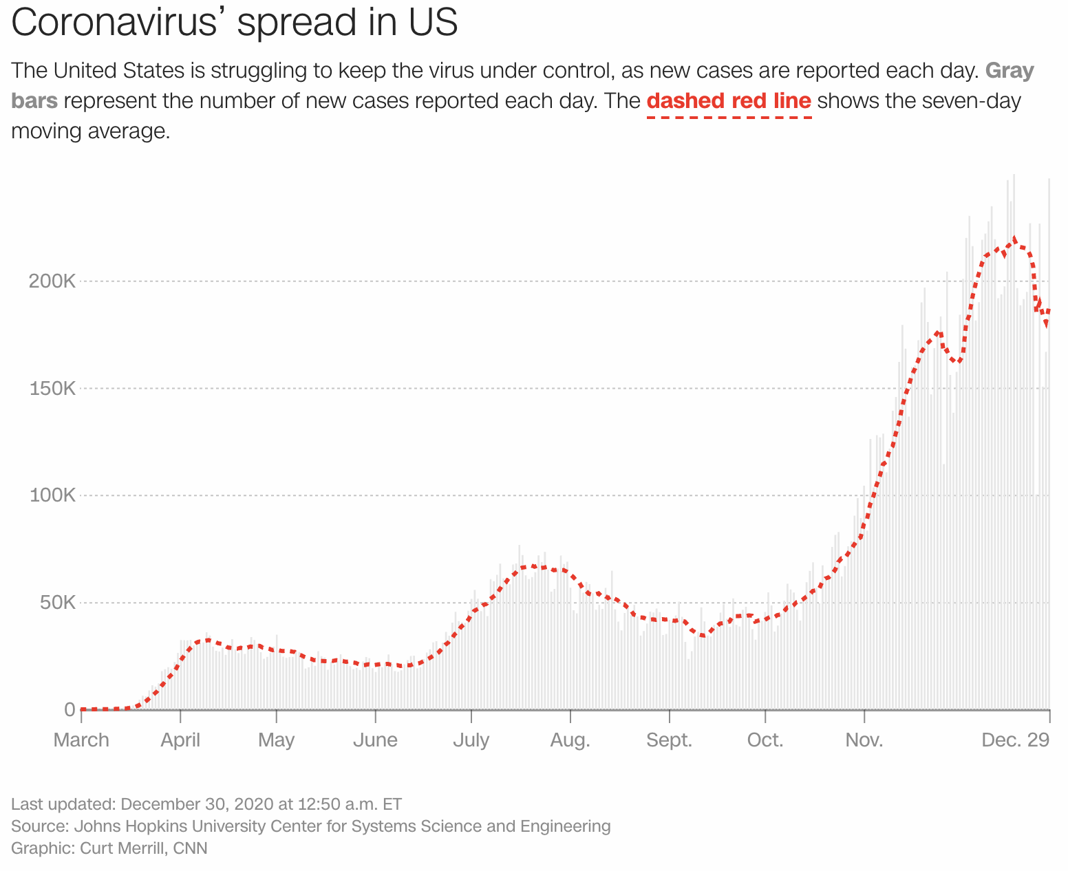
The CNN graph of covid cases on the previous page also has a seven-day moving average window overlaid on the raw data (which you can see in the faded bars). Notice how the red line makes it easier to see trends and cycles.
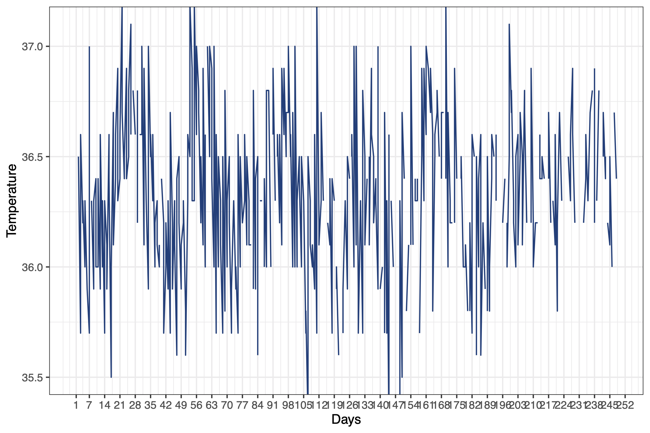
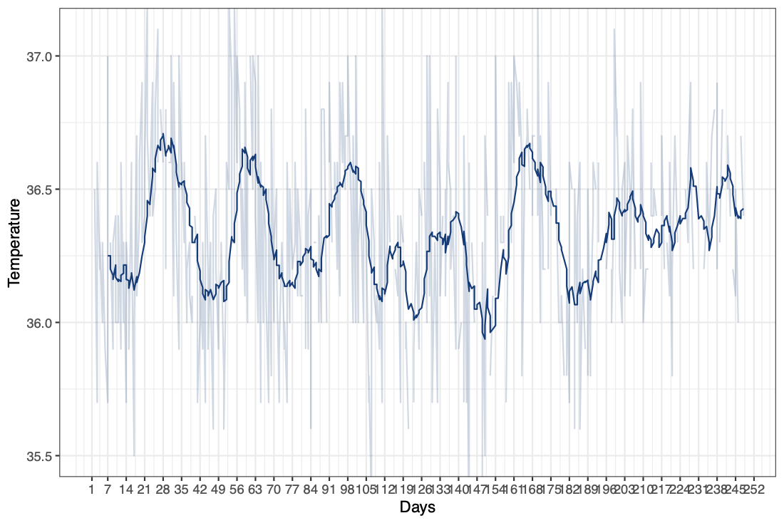
Here’s another graph that is also related to Covid. This is a real graph of body temperature, taken twice a day. Now you might not be able to see much from this data because it’s so noisy. But if we instead took a seven day moving average, we can see that this individual’s temperature data seems to follow this repeated pattern. (And indeed, this individual happens to be a female, and this data does follow a repeated, biological seasonality.)
13.2.1 Simple Moving Average Model
Now, a very simple model is to just use the window of recent values, as a prediction of the future. That is, we use the window to predict the value at the next time step: \[\hat{Y}_{t+1} = \text{Window}_t = \frac{1}{k} \left( Y_t + Y_{t-1} + \ldots + Y_{t-(k-1)} \right)\]
The major assumption in this model is that Y will stay the same, at least for short time-steps into the future. This assumes stationarity. And thus the simple moving average model does not account for trends, cycles, or seasons, and that we can get an estimate of the data just by averaging out some variation in the recent past. It’s a relatively simple model that can be calculated very quickly, even using a pen and paper pad, and can be used for quick, short-range forecasting. For example, if you are running a small store and you are wondering how much of a product to stock up on, a good estimate would be the average of those products you sold over the past few weeks.
13.2.2 Exponential Smoothing Models
The next model we’ll consider is the single exponential smoothing model. This model has a parameter called \(\alpha\). Our prediction for time \(t+1\) is a weighted sum of the actual value of \(Y_t\) and our model’s prediction \(\hat{Y}_t\). We can then subtitute in our prediction for \(\hat{Y}_t\) in terms of \(Y_{t-1}\) and \(\hat{Y}_{t-1}\), and so forth.
\[\hat{Y}_{t+1} = \alpha Y_t + (1-\alpha) \hat{Y}_{t} \\ = \alpha Y_t + (1-\alpha) \left( \alpha Y_{t-1} + (1-\alpha) \hat{Y}_{t-1} \right) \\ = \alpha \left( Y_t + (1-\alpha) Y_{t-1} + (1-\alpha)^2 Y_{t-2} + \ldots \right)\]
Thus, we end up that our model’s prediction for the next time point, \(\hat{Y}_{t+1}\), contains a weighted sum of all previous time points \(Y_t, Y_{t-1}, \ldots\). Because \(\alpha\) lies between 0 and 1, as you go further back in time, each value gets less and less weight.
So notice that there are two main differences between the simple moving average and this: this model takes into account all past data (as opposed to a finite simple moving average window), and this model gives more weight to more recent values (as opposed to the same, uniform weight in a simple moving average window).
Unfortunately, this model still doesn’t take into account trends or seasonality.
We can go further and consider a double exponential smoothing model, which can handle trends.
\[\hat{Y}_{t+k} = a_t + b_t k \]
Here we have just measured time \(t\), and now we want to forecast forward to some \(t+k\). The main idea here is that we have \(Y_{t+k}\) made up of two components, the “intercept” component \(a_t\) which “looks like” the single exponential model; and a second component, the “slope” \(b_t\) which will help it to account for trends.
\[a_t = \alpha Y_t + (1-\alpha) \left( a_{t-1} + b_{t-1} \right)\]
For the “slope” term, we have:
\[b_t = \beta \left( a_t - a_{t-1} \right) + (1-\beta) b_{t-1}\] where we update the slope estimate using both (\(a_t - a_{t-1}\)), the current slope estimate, and \(b_{t-1}\), the previous slope estimate.
The basic intuition is that each component is “smoothed” using the same linear combination (\(\alpha, (1-\alpha)\)) equation. The slope variable is also smoothed using a (\(\beta, (1-\beta)\)) equation. At every timestep we smooth and update our value of \(a_t\) and \(b_t\), using these parameters \(\alpha, \beta\) and our estimates at the previous timesteps.
There is a further generalization of this to add a third application of exponential smoothing to model seasonality. This is called the Holt-Winters model. Luckily, R’s HoltWinters() function can do all three types of exponential smoothing. The call is:
The R function will allow you to specify \(\alpha\), \(\beta\), and \(\gamma\), and whichever you do not specify it’ll try to fit.
| Method | Trend | Seasonality | Parameters | Call |
|---|---|---|---|---|
| Single Exponential Smoothing | No | No | alpha | HoltWinters(x, beta=FALSE, gamma=FALSE) |
| Double Exponential Smoothing | Yes | No | alpha, beta (trend) | HoltWinters(x, gamma=FALSE) |
| Holt-Winters | Yes | Yes | alpha, beta (trend), gamma (seasonality) | HoltWinters(x) |